Neutron reflectivity tutorial
Getting started
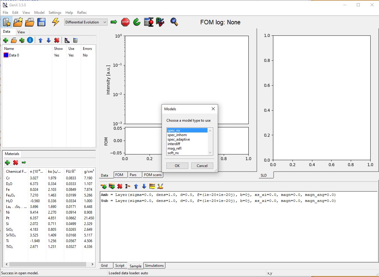
Start by opening GenX. If necessary, load the Reflectivity plugin by going to the menu . Two new tabs will appear in the lower right section of the window, Sample and Simulations. This is where we will define our sample later.
Creating a sample
Time to create the sample! Click on the Sample tab to get up our main working area at the moment. Next, create a new model by clicking on the new model button on the main toolbar (1). This will bring up a dialog window (2). Choose the spec_nx model, this includes neutron simulations.
Making a substrate
So now we have the right model to simulate neutron reflectivity. The first step is to define a substrate.
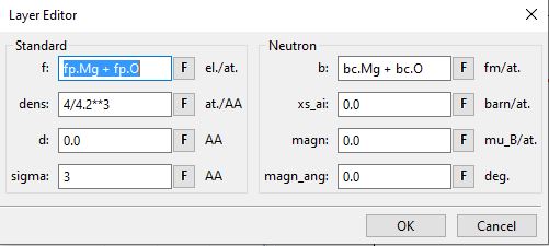
Double click on the substrate line in the list in the Sample tab, see below. This will pop up a dialog for
feeding in numbers that defines the substrate layer. Put in the same numbers as the ones below. Note that the b
box should say: bc.Mg + bc.O and in the f box should be fp.Mg + fp.O
So what does all this mean? Here is a short explanations
- b
The neutron scattering length per formula unit in fm (fermi meter = 1e-15m)
- d
The thickness of the layer in AA (Angstroms = 1e-10m)
- f
The x-ray scattering length per formula unit in electrons. To be strict it is the number of Thompson scattering lengths for each formula unit.
- dens
The density of formula units in units per Angstroms. Note the units!
- magn_ang
The angle of the magnetic moment in degres. 0 degrees correspond to a moment collinear with the neutron spin. (Only used in neutron pol spin flip calculations.)
- magn
The magnetic moment per formula unit (same formula unit as b and dens refer to)
- sigma
The root mean square roughness of the top interface of the layer in Angstroms.
Doing a simulation
Making artificial data
First we have make some x-data (q values) so we need what to simulate. Mark Data 0 in the Data tab. Next, click on the calculator above it to the right. This gives a dialog box. Choose the alternative: Simulation in the Import from, Predefined choice box. Edit it so it looks like the picture below. Click OK.

Defining the instrument
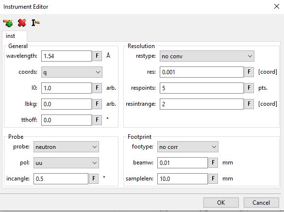
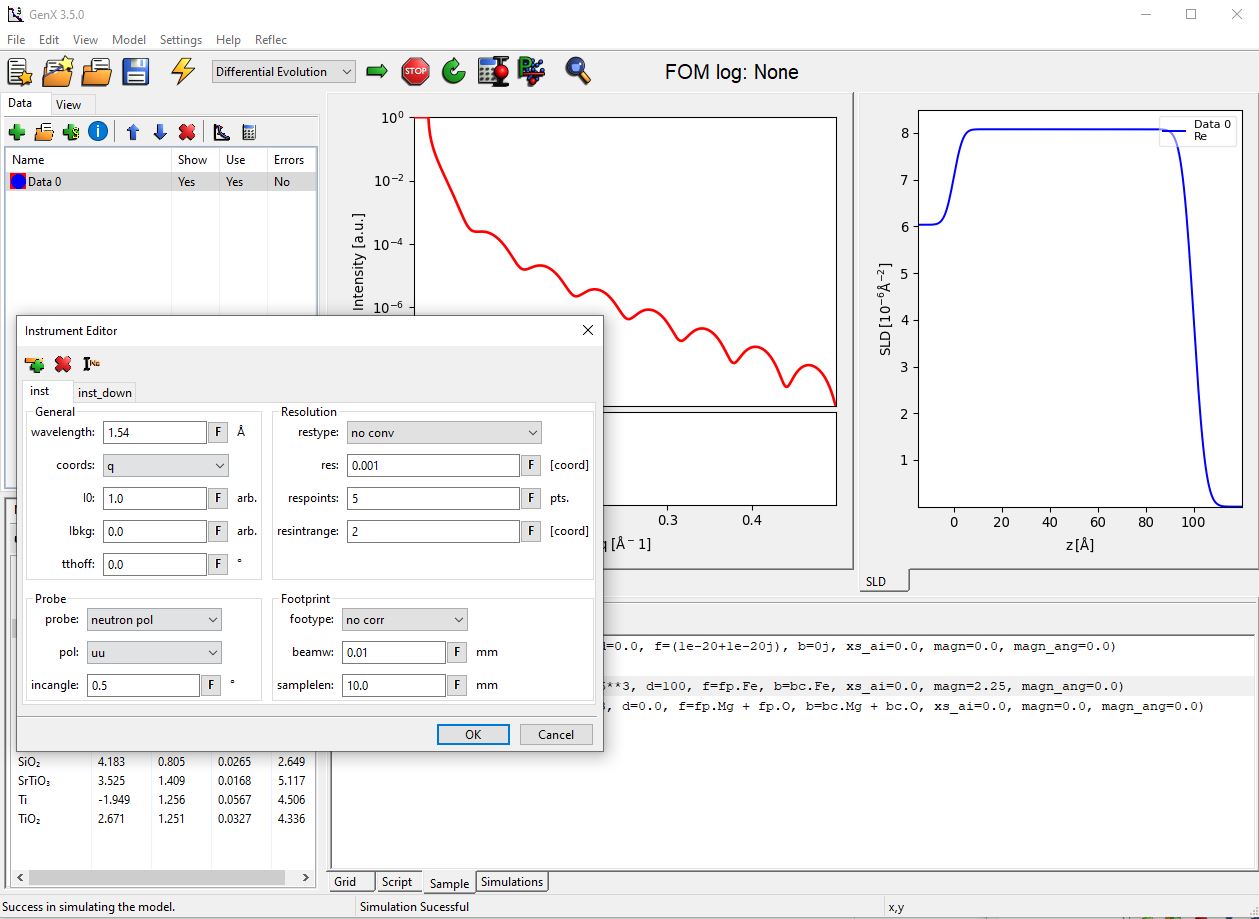
Now we have to tell the program what we mean with the data we have given it. Click on the instrument icon in the Sample tab (1). This gives the following dialog. Change the probe to neutron and coords to q. That is enough for now. Click Ok.
Simulation
Press the simulation button! (The big lightning in the main toolbar). This should produce something like this:
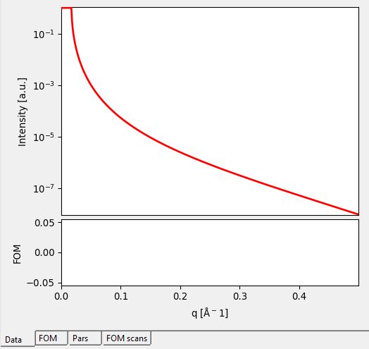
Okay, we have a total reflectivity edge. If the result is shown in linear scale, change the plot to log scale instead. Do this by going to the menu . So mission completed we have the first neutron simulation. Next step is to make a more complicated model and include polarized neutrons.
Adding Layers
Just simulating the reflectivity of a single substrate is not very fun. So, lets add another layer. Why not a magnetic, so we can play around with polarized neutron reflectivity? Before we start adding layers we have to add a stack which will contain the layers. So Add a stack by clicking on the second toolbar button in the sample tab (The one with a stack of layers and a plus). Name it to Lays for example (In the popup dialog). Now we can add a layer (First button with one layer and a plus), call it Fe for example. Look on the screenshot below for the parameters.
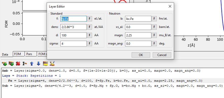
Click on the simulate button again and have look at some Kiessig fringes.
Polarized Neutron Reflectivity
Lets start the polarized neutron reflectivity by turning the polarization on in the calculations. Go to the
instrument again and choose probe: neutron pol. At the same have look at the values for the pol parameter. That is
the polarization state of the instrument: uu, dd or ud. The last one is only valid for
spin-flip calculations. Press the insert button at the top left to add a second instrument that we can
call spin_down. Here we choose equal parameters but a polarization state of dd instead of uu.
Simulate again and observe the change in the curve on the screen.
To see both polarization states at the same time, we have to add a second simulation dataset, first.
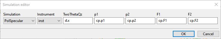
If an advanced polarization analysis experiment with determination of polarization parameters was carried out it is possible to include the non-perfect polarization in modeling with the spin-flip instrument probe parameter. You should create user parameters for the p1, p2, F1 and F2 polarization parameters as defined in https://doi.org/10.1063/1.1150060 . Then go to the Simulations tab and double click on the simulation line for a dataset. There you can select PolSpecular instead of Specular and enter the user parameters in the correct value columns. (You can also just enter the values directly, but this can be time consuming for multiple datasets.)
Adding a new data set
Add a new data set by clicking on the Add data button, the green cross above the data list. Clicking on that gives a new data set: Data 1. Mark it and click on the calculator again. Now instead of typing all that we had to the last time we import the calculations from Data 0. Click on the choice box at the top right and choose Data 0. The calculations are imported. Click on Ok.
Next, choose different plot colors for the second dataset by clicking the Plot settings button in the data toolbar and choose differnt options for the simulation (here we chose green with 4px data points). Perhaps the names are not so exciting, Data 0 and Data 1. They can be renamed by a slow double click on the name in data tab. Perhaps spin-up and spin-down is more appropriate.
Now we have to define to use the second instrument for calculations with the new dataset. Go to the simulation tab and double click on the line with Data 1. Select inst_down as Instrument from the drop down selection:
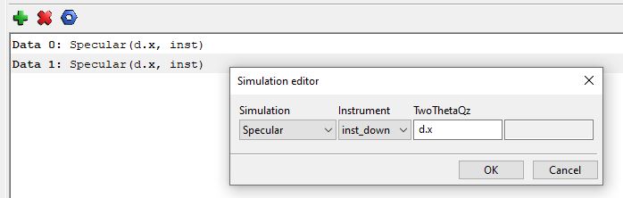
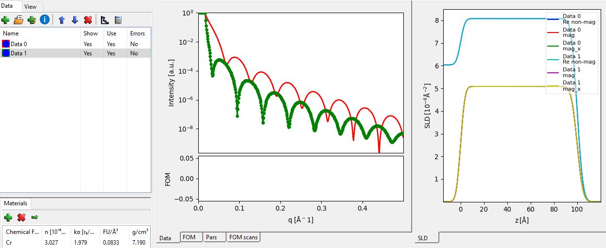
If you now simulate the data again, you should get a graph that show the splitting from the magnetic contrast in the iron layer:
Finishing off
You can, of course, do other things and not only spin polarized calculations. Perhaps simulating the x-ray reflectivity of the same sample? Just remember that the wavelength has to set as well as the probe. I guess that you can think of a couple other uses.
For information on fitting a model to data or coupling of fit parameters, have a look at the Fitting of x-ray reflectivity data. For simple models as the one described in this tutorial, the Simple Reflectivity Model (XRR/NR) can be an alternative with a much simpler user interface.