The SLD graph

The Reflectivity and SimpleReflectivity plugins add a graph to display the sample profile as height from substrate vs. scattering length density (SLD) to the user interface. There are several curves when the model is based on more then one physical propserty (real and imaginary as well as magnetic parts).

Context menu options

For the highest degree of flexibility, newer models are build to generate one set SLD profiles for each dataset as there might be changes to the model between each dataset simulation. An example would be a sample that changes thickness and density between reflectivity scans or a change in magnetization profile for different external fields or temperatures. On the other hand this feature can lead to a large number of curves that become hard to read. The context menu (right click on graph) therefore provides additional options to change the plot display:

• Legend Outside

  Reduces the plot area and places the line legend on the right of the graph instead of in the top-right corner.

• Color from Data

  Uses the simulation color of each dataset to define SLD graph colors. The possible items that make up each simulation are derived by changing the color saturation and value (HSV).

• Single Sample Mode

  For simulations that do not change the sample model between datasets this can be activated to display just the SLD profile of the first simulation.

SLD uncertainty

With the Reflectivity plugin the SLD profile can also be used to visualize the parameter uncertainties from a fit. While this results in an intuitive display of real-space geometry one has to keep in mind that reflectometry does not measure the geometry directly but correlations between interfaces and the results are thus translation invariant. The user will therefore have to choose a reference interface that is kept fixed for this modeling.

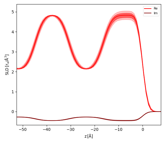
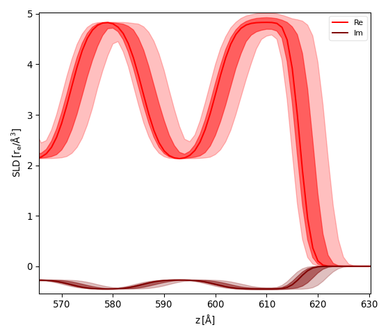
After fitting the model and caluculating the errors on parameters (see Error Statistics from bumps library) activate the menu Reflec‣Uncertainty Profile…. A dialog will ask to enter the reference interface (python style index 0=Substrate, -1=Surface) and the number of samples. GenX will then simulate your model while choosing number of samples random parameter sets choosen from a gaussian distribution. The SLD will be calculated for the reference interface at z=0 and the SLD plot will show the fit result (line) together with two bands of uncertainty as partially transparent curves. The stronger curve is the 1-sigma (68.2%) and the more transparent the 2-sigma (95%) interval.

The pictures below show the result for the x-ray reflectivity example close to the sample surface using a reference surface of -1 (left) and 0 (right):

Custom filter

If the buildin options to display the profiles do not fit your needs you can modify the displayed datasets and components within the model script. The recent reflectivity model Sim function will start like this:

SLD = []
def Sim(data):
    I = []
    SLD[:] = []
    # BEGIN Dataset 0 DO NOT CHANGE
    d = data[0]
    I.append(sample.SimSpecular(d.x, inst))
    if _sim: SLD.append(sample.SimSLD(None, None, inst))
    # END Dataset 0

If the model ist simulated (not fit) the _sim variable will be set to True resulting in the global list SLD to be populated. It will have one entry for each dataset in the model. Each entry (retuned by sample.SimSLD) is a dictionary containting each of the SLD lines as well as the z-values and the SLD unit. The dictionary keys are used in the plot legend, so you can see in the graph which items carry the information that is relevant.

To remove certain datasets or SLD lines from the graph, add a filter at the end of the Sim function:

if _sim:
    for i in [1,3,5]:
        SLD[i]={}
    for i in [2,4]:
        del(SLD[i]['Re non-mag'])

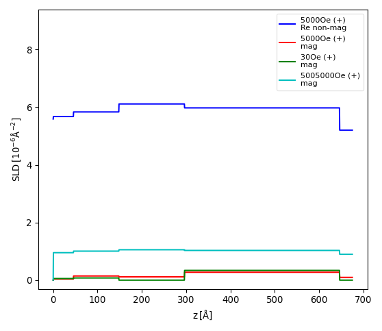
The example above is taken from a neutron reflectivity fit of 6 datasets, with even numbers being spin-up and odd numbers spin-down. The first for-loop removes any lines from the spin-down channels, as the model does not change between these datasets. The second for-loop removes the non-magnetic SLD part for dataset 2 and 4. The resulting graph is shown below:

Note

This user filtering is not supported by the SLD export facility that expects all information for each of the datasets. Before exproting SLD you should thus comment out this section and simulate the data again.