Data handling

Adding/Removing

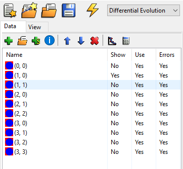
A data set can be added by using the green cross above the list of data sets in the data tab (leftmost notebook), see picture above. In the same manner one or several data sets can be deleted (no undo) by pressing the red cross next to the blue arrows. A dialog will appear to make sure that you really want to remove the data set. The data sets can also be moved up and down in the list by using the two blue arrows.

It is possible to change the name of the current data set in order to make it more human readable. This is done by double clicking or clicking twice (platform dependent, I believe) on the dataset name. You can look at possible meta data that was imported by pressing the blue information button.

Lastly, the three different columns after name in the data list shows the status for each data set with regards to plotting and fitting. The following list will explain them:

Show

Whether or not to plot the dataset in the plot window. If Yes it will be plotted.

Use

If the dataset should be used to calculate the Figure of merit FOM. If Yes it is used. This is for fitting.

Use Error

If the error bars on the data should be used in both plotting and fitting. The fitting part only works if the FOM function supports it, i.e. Chi2 functions and similar. The error bars will only be displayed when the data is simulated. During fitting they will not be shown due to performance issues with the plotting.

These states can be toggled (switched between yes and no) by right clicking on the data set and choose the right menu item in the pop-up menu.

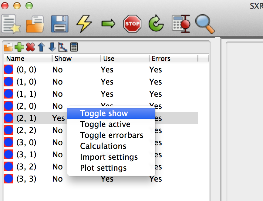
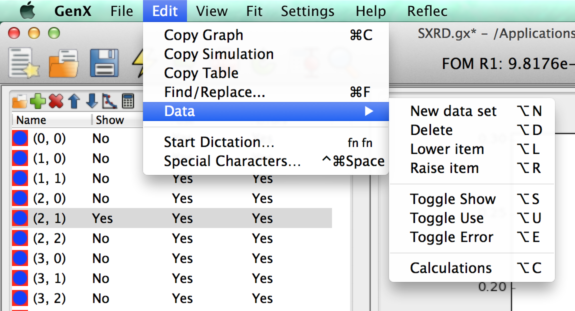
There are also keyboard shortcuts for these if you need to access them frequently, see the menu Edit‣Data.

Loading

Before loading data you should choose which data set to load the data into. This is done by simply marking the data set in the list. Some loader support multiple datasets, if they are present in the file. To load data click on the folder icon in the data tabs upper toolbar. This will open up a file dialog that allows you to choose which file to load. Note that the behavior could be customized if you use a different data loader plugin, see Overview of the user interface.

As a default the data to load is assumed to be two column ASCII format with the columns of x and y data separated by any whitespace character, i.e., spaces and tabs. A comment should be preceded by a hash(#). If you would like to change these parameters you can right click on any data set and choose Import settings from the pop-up menu to change the behavior. It is also possible to choose Settings‣Data Loader from the pull-down menu. This will make a dialog window to appear where the data loading process can be customized. Here one should note that all columns and numbered 0, 1, 2 ….

Note

The numbering starts with 0!. Internally the numpy loadtxt function is used.

Viewing

As soon as a data set has been loaded this should be displayed in the main plot. If that is not the case something has gone wrong. In these cases, and others too, the data can be viewed from the view tab in the leftmost notebook panel. There are several columns here and the x_raw, y_raw, ye_raw represents the data as loaded directly from the source file. The last column represents the displayed value after any Calculations/Transformations have been applied to the data, see next section.

Calculations/Transformations

Here some useful expressions for treating the raw data are presented. The treatment can be defined by clicking on the calculator button on the data toolbar to access the Data Calculations dialog, see below.

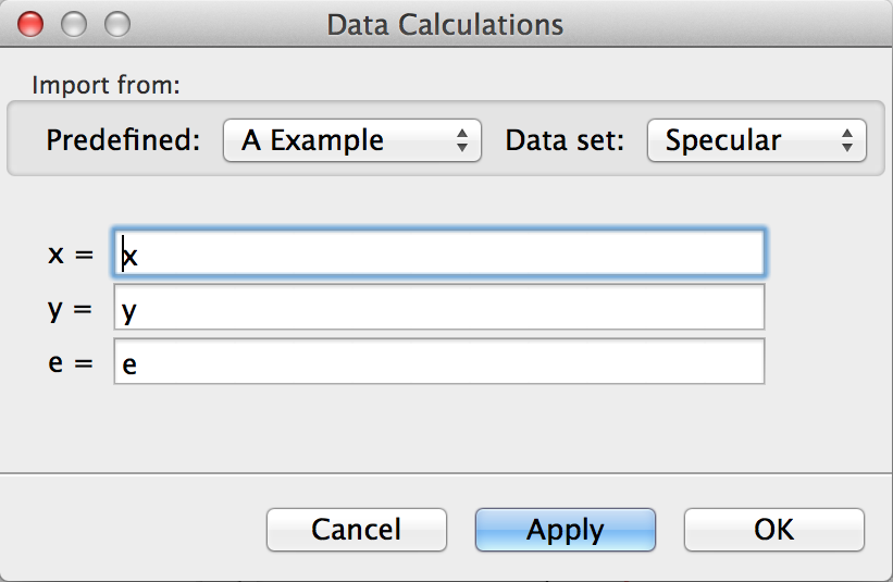
Any Python expression will work. (Based on numpy arrays.) First of all to reset the data to the raw data write, x in the x field and y in the y field. The general syntax for selecting data from an array is:

x[start:end:step size]

If a special interval of the data needs to be fitted:

x[20:-300]

where the first value is the starting point (number of elements from the beginning) and the last is the end point. A negative value means that the end point is calculated from the end of the array. In addition, if the number of data points has to be decreased the expression above can be extended to include the step size:

x[20:-300:2]

For more information about indexing see. Consequently with this expression only every second data point is included. The operations shown here also need to be performed on the y,error and any extra_data values.

It is also possible to conduct simple arithmetic operations on the data. For example transforming the x data from degrees to Qz (scattering vector in reciprocal Angstrom), assuming that a wavelength of 1.54 Å is used:

4*pi/1.54*sin(x*pi/180)

This would then be typed into the text field for the x data.

Another common action is to calculate counting errors based on the input data. For data that is imported directly in the unit of counts one would put into the e entry:

sqrt(y)

Note

Three special functions are provided by GenX for advanced data treatment. These are:

• rms(e1,e2,e2,…) calculates the Root Mean Square of a set of error values. This is useful when combining statistical errors from different sources. (Like the ones calculated withe the two functions below.)

• fpe(max_x,rel_e) get the estimated foot print error that results from imperfect beam homogenity in a angular-dispersive reflectivity experiment. Providing a relative error rel_e and maximum x-value with footprint influence max_x the absolute error on y is calculated.

• dydx() calculates the numerical slope dy/dx for each datapoint. This can be used to estimate an error on the simulated intensity that results from an error on the data-point x location by multiplying with the standard deviation of the x-value.

Use Predefined‣Systematic Errors to see an example use for an XRR measurement with 1° maximum footprint, 2% relative footprint error and 0.01 standard deviation of x-values for all points.

The examples presented here are rather limited but hopefully to shows the flexibility of treating the data. For a more detailed list of functions and syntax the reader is referred to the tutorials and manuals found at scipy.

Exporting

Data can be exported to four-column ASCII format (x, y, y_err, simulation) by using the menu File‣Export‣Export Data and choosing a data name. Each dataset will be saved to an individual file with a running number from 000, 001 … and upwards inserted before the given extension. For example, if the name export.dat is given the output files will have the names export000.dat, export001.dat and so on.

GenX now supports the new ORSO Open Reflectometry Text (.ort) ASCII format with additional metadata from the imported datasets and GenX model. All datasets are included in a single text file by using the menu File‣Export‣Export ORT and choosing a file name as export.ort.

Also, if you want to plot the data in another plotting program, such as Gnuplot, Excel, OpenOffice or Origin. The data can be copied in a ASCII spreadsheet format directly to the clipboard. This is done by using the menu Edit‣Copy Simulation. This will make all data sets in 4-column format after each other, column-wise.